

PythonPro #5: Snowflake LLMs, Pandas Creator at Posit, Jupyter notebooks, and more
Bite-sized actionable content, practical tutorials, and resources for Python programmers

“When you teach them - teach them not to fear. Fear is good in small amounts, but when it is a constant, pounding companion, it cuts away at who you are and makes it hard to do what you know is right.”
― Christopher Paolini (2011), Inheritance
Is fear a bug or a feature in your Python coding journey? Welcome to this week’s issue of PythonPro!
In today’s Expert Insight section we dive into an excerpt from Hands-On Application Development with PyCharm - Second Edition 📘 to explore how Jupyter notebooks revolutionize data analysis, and how PyCharm supports your iterative development process.
But that's not all – we've got a wealth of Python updates, case studies, tutorials, and more waiting for you including:
🔍Python Pandas creator Wes McKinney joins Posit as principle architect
📦An unbiased evaluation of Python environment management and packaging tools
🎥Automatically determine video sections with AI using Python
Stay awesome!
Divya Anne Selvaraj
Editor-in-Chief
P.S.: If you want us to find a tutorial for you the next time or give us any feedback, take the survey and as a thank you, you can download a free e-book of the Python Feature Engineering Cookbook. This survey will expire on 14th November, 2023.
🐍 Python in the Tech 💻 Jungle 🌳

🗞️News
Snowflake puts LLMs in the hands of SQL and Python coders: Snowflake has introduced a fully managed service, Snowflake Cortex, for developers to easily implement LLMs in data-driven applications, without the need for complex AI expertise and GPU infrastructure management. Read to learn more about the service’s benefits including how it simplifies tasks like sentiment analysis.
Python Pandas creator Wes McKinney joins Posit as principle architect: Posit, formerly RStudio, is broadening its mission to support data science practitioners in both R and Python, with initiatives like the Shiny Web framework for Python, the Quarto publishing platform, and the Posit Connect enterprise data platform for collaboration in both languages. Read to learn how McKinney plans to champion the PyData ecosystem and advance open-source projects in this new role.
Apache 3.5 boosts Python UDF Performance with Arrow Optimization: This optimization significantly improves user-defines function (UDF) performance, making data exchange between JVM and Python processes faster and more reliable. Read to learn how arrow optimization improves (de)serialization speed and enables standardized type coercion, and go through practical examples for implementation.
💼Case Studies and Experiments🔬
Python Case Studies and Success stories by the PSF: This collection of case studies highlights Python's impact on various fields, including web services, GIS, earthquake risk assessment, and more using real-world success stories. Read to learn why Mozilla and Bitly rely on Python for web services, why Python is used by Google to power its mission of organizing the world's information, and a lot more.
📊Analysis
An unbiased evaluation of Python environment management and packaging tools: This article evaluates these tools and categorizes them into five key areas: Python version management, package management, (virtual) environment management, package building, and package publishing. Read to find out which tools excel in dependency management, project metadata compliance, and more.
A Comparative Analysis of Different Python Editors: This study compares 8 popular Python editors including Spyder, VSCode, Atom, PyCharm, Sublime Text3, IDLE, and Jupyter Notebook. Comparison parameters include speed, cost, project complexity, scalability, level of programming experience, customizability, flexibility, and more. Read for an in-depth evaluation of each editor's strengths and weaknesses and to be able to choose the right one for your needs.
🎓 Tutorials and Guides 🤓

Python Packaging User Guide: This is a valuable resource to Learn the ins and outs of packaging, including tool selection and processes tailored to your needs. Read for tutorials for package installation, managing dependencies, and distribution; expert guides for specific tasks; and more.
Let's Code a Wicked Cool Calculator: This tutorial will guide you through creating a feature-packed calculator using Tkinter for the GUI, sympy and matplotlib for math problem solving, and pytesseract for image-to-text extraction. Read if you're interested in enhancing your coding skills and want to delve into practical Python application development using a step-by-step guide.
Is manually creating HTML tables a hassle for you?: This article will teach you how Django Tables2 lets you define tables in Python and have Django render them effortlessly. Read to also learn how to add htmx for dynamic loading, sorting, and pagination, all without writing complex JavaScript.
Get started using Python for web development on Windows: This guide will help you kickstart Python web development with Windows Subsystem for Linux (WSL). Read to learn how to set up the WSL, configure Visual Studio Code, create a virtual environment, and develop web applications with Python, Flask, and Django using WSL and Visual Studio Code.
Automatically determine video sections with AI using Python: This detailed tutorial covers video segmentation, generating section titles with LLMs, and formatting the information for YouTube chapters. Read if you are considering sharing coding or data science wisdom on YouTube and get set up to automate video segmentation and enhance video content using Python.
🔑 Best Practices and Code Optimization 🔏

How Can DS-1000Enhance Your Python Data Science Code Generation?: DS-1000 is a benchmark for testing how well computer programs can generate code for data science tasks. It includes a thousand real-world problems from sources like Stack Overflow, covering 7 Python libraries like Numpy and Pandas. The benchmark is unique because it has three important qualities: it includes a wide variety of practical problems, it evaluates code accuracy very precisely, with only1.8% of predictions being wrong, and it defends against memorization. Read the entire paper documenting the development of the benchmark here or access the benchmark directly here.
Fortifying Python Web Apps: Cybersecurity Best Practices: This research paper offers a tailored guide for securing Python web applications, covering common vulnerabilities and mitigation strategies. It delves into Web Application Firewalls (WAFs) and Intrusion Detection Systems (IDS), stresses continuous security testing, and more. Read to pick up best practices and examine real-world cases that reveal the consequences of lax security.
7 Tips to Structure your Python Data Science Projects: This video guide will teach you how to improve your project management and coding practices with seven tips, including using a common project structure, leveraging existing libraries, organizing reusable code, and more. Watch if you want to streamline your projects with robust code.
Making PySpark Code Faster with DuckDB: DuckDB provides a lightweight alternative to resource-intensive Apache Spark for smaller pipelines and local development, offering PySpark API compatibility to reduce container image size and enhance processing speed. Read to learn more about this approach which is still experimental but shows promise in optimizing data processing tasks.
Optimizing Timestamp Functions in Python: Performance Insights and Best Practices: This article analyses and compares the performance of various Python timestamp functions including time.time(), datetime.now(), datetime.utcnow(), and pytz-based functions. Read for insights which demonstrate that generating UTC timestamps is faster, advise on when to use different timestamp functions, and learn about the minimal overhead of datetime objects.
🧠 Expert insight 📚

Here’s an excerpt from “Chapter 12, Dynamic Data Viewing with SciView and Jupyter” in the book Hands-On Application Development with PyCharm - Second Edition by Bruce M. Van Horn II and Quan Nguyen.
Leveraging Jupyter notebooks
Jupyter notebooks are arguably the most-used tool in Python scientific computing and data science projects. In this section, we will briefly discuss the basics of Jupyter notebooks as well as the reasons why they are a great tool for data analysis purposes.
Then, we will consider the way PyCharm supports the usage of these notebooks.
We will be working with the jupyter_notebooks project in the chapter source. Don’t forget you’ll need to install the requirements within the requirements.txt file in a virtual environment in order to use the sample project. If you need a refresher on how to do this, refer back to Chapter 3.
Even though we will be writing code in Jupyter notebooks, it is beneficial to first consider a bare-bones program in a traditional Python script so that we can fully appreciate the advantages of using a notebook later on. Let’s look at the main.py file and see how we can work with it. We can see that this file contains the same program from the previous section, where we randomly generate a dataset of three attributes (x, y, and z) and consider their correlation matrix:
import pandas as pd
import numpy as np
import matplotlib.pyplot as plt
# Generate sample data
x = np.random.rand(50,)
y = x * 2 + np.random.normal(0, 0.3, 50)
z = np.random.rand(50,)
df = pd.DataFrame({
'x': x,
'y': y,
'z': z
})
# Compute and show correlation matrix
corr_mat = df.corr()
plt.matshow(corr_mat)
plt.show()
This is roughly the same code we used earlier in this chapter when we wanted to expose the heatmap features in PyCharm when reviewing a correlational matrix. Here, we have added the last two lines, which are different. Instead of a heatmap, this time we’re drawing a scatter plot. I explained earlier that we have intentionally and artificially introduced correlation into our otherwise randomly generated data. Examine where we set y and you’ll see we multiplied the matrix from x by 2, then added some small numbers from another random sample generation. This will make y appear to be roughly, but not exactly, correlated to x allowing us to see a plausible, though contrived, correlation matrix. This proves out when we run the file. My result is shown in Figure 13.24. Don’t forget that our data is random, so yours will not precisely match mine.

Figure 13.24: This is the scatter plot produced by our code
Like I said, there’s nothing new or amazing here besides the change from a heatmap to a scattelot. We ran this as a point of comparison for our discussion of Jupyter notebooks.
Understanding Jupyter basics
Jupyter notebooks are built on the idea of iterative development. In any development effort regardless of what you are creating, breaking a large project into smaller pieces always yields rewards. Nobody at the Ford Motor Company just builds a car. They build millions of pieces that are later assembled into a car. Each piece can be designed, produced, tested, and inspected as individual pieces.
Similarly, by separating a given program into individual sections that can be written and run independently from each other, programmers in general and data scientists specifically can work on the logic of their programs in an incremental way.
The idea of iterative development
Most practitioners in the world of software development are used to the ideals behind agile methodologies. There are dozens of agile frameworks designed to help you manage software, or really, any project with the aim of creating some useful product. One thing they consistently have in common is the idea of iterative development. The development effort is broken down into smaller, simpler tasks called an iteration. At the end of each iteration, we should have some usable product. This is important!
You might think about making a car, but think truly about the research and development that went into the first cars. Our main concern at that time was to produce a vehicle to take us from point A to some distant point B in a manner that was faster and more efficient than using a domesticated animal.
We already know about the wheel, so let’s entertain at a somewhat comical level the process your average software developer might use if they were going to create the world’s first automobile. Remember, each iteration must produce some usable means of traveling from place to place. Our development team might start with a skateboard. This is something simple we could make in a short iteration. The next iteration might produce a scooter, the next a bicycle, the next might be a powered tricycle, then eventually, a rudimentary car. See Figure 13.25.

Figure 13.25: An iterative process realizes a goal one step at a time
Each iteration produces a usable result, and we can point to this as continuous progress. At the end of each iteration, you should reflect upon the next because, with each iteration, your understanding of the final objective becomes clearer. You learn a lot from each iteration, and if you keep your iterations small, you have the flexibility to change direction when you discover you need to.
This happens all the time in traditional software development and in data science work. You may set out with a particular research objective in mind, but ultimately, you have to go where the data leads you rather than succumbing to your own bias. Iterative processes make this possible.
We can apply this to the ideas behind Jupyter notebooks since these involve building up your work one cell, or iteration, at a time. During each iteration, you add or make the appropriate changes in the code cell that reads in the dataset and rerun the subsequent cells, as opposed to rerunning the code before it. As a tribute to its users, Jupyter notebooks were named after the three most common scientific programming languages: Julia, Python, and R.
Another integral part of Jupyter notebooks is the support for the Markdown language. As we mentioned previously, at the beginning of the previous chapter, Markdown is a markup language that’s commonly used in README.md files in GitHub. Furthermore, because of its ability to work with LaTeX (which is typically used for writing mathematical equations and scientific papers in general), Markdown is heavily favored by the data science community.
Next, let’s see how we can use a Jupyter notebook in a regular PyCharm project
Jupyter notebooks in PyCharm
For this task, we will be translating the program we have in the main.py file into a Jupyter notebook so that we can see the interface that Jupyter offers compared to a traditional Python script. I’ll be leveraging my existing jupyter_notebooks project we started with. You can find it in the chapter’s sample code. If you don’t have that repository, we cover cloning it in Chapter 2. If you’d like to start from scratch, you can simply create a new scientific project, which was covered in Chapter 12.
Creating a notebook and adding our code
To add a new Jupyter notebook in a PyCharm project, create it as though it were just a file. Click File | New | Jupyter Notebook as shown in Figure 13.26.

Figure 13.26: Create a new Jupyter notebook using the File | New menu option
You are immediately prompted to name your notebook. I called mine basic.ipynb. The file was created in the root folder of my project, but I went ahead and dragged it into the notebooks folder…
Let’s begin by typing some documentation along with some known imports. At the prompt, type this code:
### Importing libraries
import pandas as pd
import numpy as np
import matplotlib.pyplot as plt
#%%
When you type the last #%%, you’ll find PyCharm starts a new cell for you. In the second cell, let’s enter some of the code we had earlier in our illustrative Python script:
x = np.random.rand(50,)
y = x * 2 + np.random.normal(0, 0.3, 50)
z = np.random.rand(50,)
df = pd.DataFrame({
'x': x,
'y': y,
'z': z
})
#%%
I’ve explained this code earlier in this chapter, so I won’t do that again. As before, the last #%% will create a new cell. See Figure 13.28 to see what I have so far.
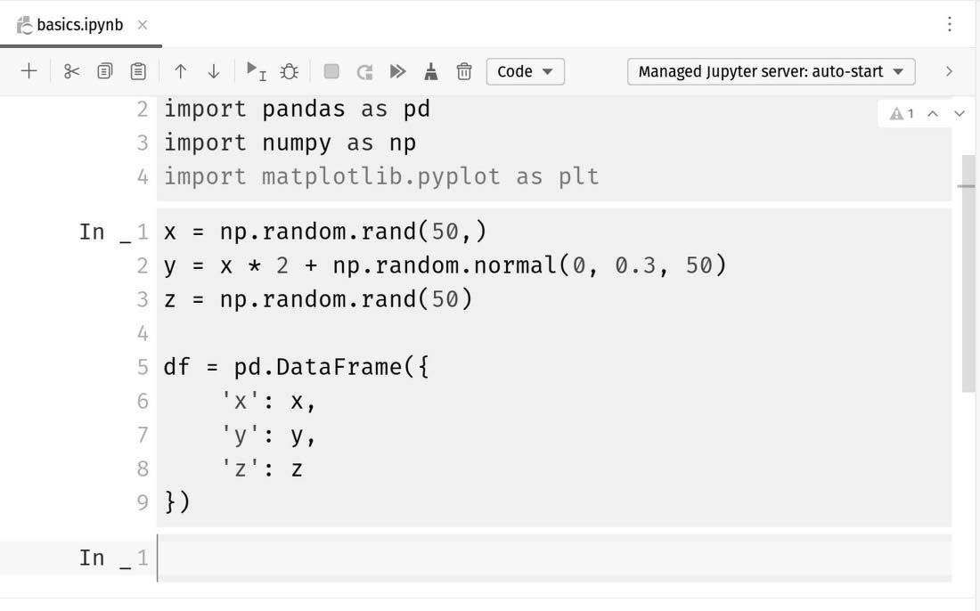
Figure 13.28: I now have two cells containing our code from our earlier program
So far so good! I have my imports and a cell that generates my dataset for me just as I had in my Python script. I’ve been breaking my program up into small, iterative steps. First, my imports, then my dataset. Next, I can look at doing something with my data. We know from earlier discussions that this is going to be a correlative matrix. What if this is a university project, and our professor wants us to document the formulae we use? That’s probably a good idea even if you’re out of school. Let’s take a moment to look at a cool documentation feature we can use. We know we can have code cells. We can also have documentation cells that leverage not only Markdown but also LaTeX.
Documenting with Markdown and LaTeX
…
Let’s try it out!
First, I haven’t been totally up-front with you on how to create cells. Sure, you can just start typing stuff in, and using #%% to separate cells works just fine. You can also hover over the space between cells, or where the division would be if you’re at the top or bottom of the notebook. Check out Figure 13.29.

Figure 13.29: You can hover in the space between cells to get a little GUI help with adding new cells
When you click these buttons between cells, it triggers a process of cell division called mitosis. Wait, no, that’s biology. It does split the cells by adding a new one between the two we have. I’m going to add a cell below my last one by hovering just below the last cell and clicking Add Markdown Cell.
This will create a light blue cell without the IPython prompt. Since it’s a Markdown cell, PyCharm isn’t expecting code, so there’s no need for the prompt. Now, within the cell, type this absolute nonsense:
### Pearson's correlation
$r_{XY}
= \frac{\sum^n_{i=1}{(X_i - \bar{X})(Y_i - \bar{Y})}}
{\sqrt{\sum^n_{i=1}{(X_i - \bar{X})^2}}\sqrt{\sum^n_{i=1}{(Y_i - \bar{Y})^2}}}$
This is LaTeX markup syntax that will convey Pearson’s formula for correlation. Trust me, it will be quite impressive in just a moment when we run our notebook. Let’s go ahead and add our two plots from earlier.
Adding our plots
Add a new code cell below the last one and add this code for our heatmap:
# Compute and show correlation matrix
corr_mat = df.corr()
plt.matshow(corr_mat)
plt.show()
Next, add another code cell for our scattelot:
# Scatterplot
plt.scatter(df['x'], df(['y']))
plt.show()
Our implementation of our code as a Jupyter notebook is complete.
Executing the cells
You can execute the notebook by clicking the run button at the top of the notebook...
This triggers a marvelous transformation in PyCharm…
First, notice there is a new tool on the left sidebar for Jupyter. We can see we’ve started a Jupyter server running on port 8888. If you were using Jupyter independently of PyCharm, this would be the normal mode of operation. You’d have run the Jupyter server from the command line and navigated to the notebook in your browser. PyCharm is replacing that experience within the IDE, but we still need to run the server to get the results.
If you scroll up, you’ll see the LaTeX markup has been rendered in our Markdown cell shown in Figure 13.33.

Figure 13.33: The nonsense now looks absolutely stunning!
If you scroll down to inspect the scatterplot, we see… Well phooey! There’s an error!

Figure 13:34: The error message shows us exactly what is wrong
I messed up. I put parentheses alongside the DataFrame object, df. I need to take those off so it looks like it’s a neighbor:
# Scatterplot
plt.scatter(df['x'], df['y'])
plt.show()
Now, I could rerun the whole notebook, but I don’t need to. The problem was in the last cell, so I could just put my cursor in the last cell and click the single green run arrow. See Figure 13.35.

Figure 13.35: Yes, that’s much better!
…
We have gone through the main features of PyCharm in the context of Jupyter notebooks. In general, one of the biggest drawbacks of using traditional Jupyter notebooks is the lack of code completion while writing code in individual code cells. Specifically, when we write code in Jupyter notebooks in our browser, the process is very similar to writing code in a simple text editor with limited support.
However, as we work with Jupyter notebooks directly inside the PyCharm editor, we will see that all the code-writing support features that are available to regular Python scripts are also available here. In other words, when using PyCharm to write Jupyter notebooks, we get the best of both worlds—powerful, intelligent support from PyCharm and an iterative development style from Jupyter.
Hands-On Application Development with PyCharm - Second Edition by Bruce M. Van Horn II and Quan Nguyen was published in October 2013 and is a valuable resource for both Python web developers and data scientists.
And that’s a wrap.
We have an entire range of newsletters with focused content for tech pros. Subscribe to the ones you find the most useful here. The complete PythonPro archives can be found here.
If you have any comments or feedback, take the survey or leave your comments below!
See you next week!