

PythonPro #9: Django 5.0, Hugging Face API Security, and Advanced Geospatial Analysis

“If the implementation is hard to explain, it's a bad idea.
If the implementation is easy to explain, it may be a good idea.”
— Tim Peters (2004), The Zen of Python
Welcome to a brand new issue of PythonPro!
Highlights: Django 5.0 is out with game-changing features. Hugging Face's API exposure fiasco underscores the urgency of securing AI and ML supply chains. Also, an open letter from Python Africa, reveals concerns about grant delays and biases that negatively affect non-western Python events.
We've also got a fresh batch of tutorials and tricks and here are my top 5 picks:
Building Predictive Models Using Logistic Regression in Python🔍
📑Job Queues With Postgres - A working example with async Python and Quart
In today’s Expert Insight section we have an exclusive excerpt from the book Learning Geospatial Analysis with Python - Fourth Edition, that will teach you advanced geospatial analysis through a Python implementation of least cost path analysis to optimize routes through varied terrains. So dive right in!
Stay awesome!
Divya Anne Selvaraj
Editor-in-Chief
P.S.: If you want us to find a tutorial for you the next time or give us any feedback, take the survey and as a thank you, you can download a free e-book of Interactive Data Visualization with Python - 2nd Ed..
🐍 Python in the Tech 💻 Jungle 🌳

🗞️News
Django 5.0 released: The news release features database-computed default values, generated model fields, and field groups in templates. Read to learn more and understand why it is important to upgrade to version 4.2 or later.
Exposed Hugging Face API tokens offered full access to Meta's Llama 2: Hugging Face, known for its Transformers Python library, inadvertently exposed over 1,500 API tokens, including those of tech giants like Meta, Microsoft, Google, and VMware, posing a potential risk of supply chain attacks. Read to learn more and understand the critical need for securing AI and ML supply chains.
An Open Letter to the Python Software Foundation from Python Africa: This letter from DjangoCon Africa organizers highlights frustrations with the PSF's delayed $9,000 grant and internal biases, and calls for transparency and collaboration to address issues affecting non-western Python events. Read to understand the challenges faced by non-western Python events and their impact.
💼Case Studies and Experiments🔬
Pandas Live Case Study on Uber Cab Data: This advanced Python session offers a comprehensive guide to data cleaning, transformation, and insightful analysis for Python practitioners. Watch to learn how to discover patterns, monthly trends, and develop expertise in real-world data manipulation.
Building a semantic search engine in Python: This article explores building a semantic search engine in Python, debunking the misconception that it requires complex tools. Read for a practical guide to using neural networks, Python code, and efficient scaling strategies to enhance your search capabilities.
📊Analysis
Navigating an AMD CPU Bug's Impact on FSRM and System Calls in Rust, Python, and C: This article explores the unexpected performance disparity between Rust's std fs, Python, and C due to an AMD CPU bug related to FSRM (Fast Short REP MOV). Read for an insightful investigation using tools like strace, perf, and eBPF.
Climbing Mount Everest in Flip-flops: My journey into PHP as a Python dev: This article chronicles a Python developer's immersive journey into PHP by crafting a printing API with Cody, an AI assistant. Read to explore how AI tools can streamline and accelerate the learning curve for developers transitioning between programming languages.
🎓 Tutorials and Guides 🤓

Build Conway's Game of Life With Python: This tutorial covers algorithm implementation, curses view creation, and CLI app development to enhance your object-oriented and command-line skills. Read if you are interested in object-oriented Python, CLI apps, and project setup.
Making ChatGPT hear and talk with Python: This tutorial will help you build a voice-enabled ChatGPT that you can use even on your browser, using Whisper API for speech-to-text and Chat Completion API. Watch for a step-by-step coding guide to create a personalized voice interface.
A Smooth Transition from Excel to Python: This article explores the integration of Mito, a powerful spreadsheet tool, with Dash applications, to enable a seamless transition for Excel users to Python. Read if you want to up your analytics game with an Excel-like interface, simplify app development, or automate manual tasks.
Structural Pattern Matching Tutorial: This comprehensive guide will help you master Python's pattern matching syntax introduced by PEP 634. Read to learn about topics such as sequence matching, handling specific values, composing patterns, and advanced techniques for capturing sub-patterns and matching against constants.
Building Predictive Models Using Logistic Regression in Python: This tutorial delves into logistic regression for machine learning, covering theory, mathematics, and practical coding in Python. Read for a hands-on demonstration using the scikit-learn library on the Ionosphere dataset for effective model building and evaluation.
Visualizing Evoked data: This tutorial explores diverse visualization methods for Evoked data in MNE-Python, covering butterfly plots, spatially colored traces, scalp topographies, arrow maps, joint plots, comparison across conditions, and more. Read to make informed decisions in neuroimaging or if you are interested in signal processing and visualization techniques.
Data Visualization: How to Choose the Right Plots with Plot Interpretation: This article demystifies data visualization, guiding you through the selection of appropriate plots for different data types. Read to navigate through numerical and categorical variables with clarity and elevate your data storytelling skills.
🔑 Best Practices and Code Optimization 🔏

Job Queues With Postgres - A working example with async Python and Quart: This article explores the implementation of job queues with Postgres, async Python, and Quart, emphasizing efficient scheduling, execution, and testing strategies. Read to learn how to leverage the SKIP LOCKED feature for seamless job handling and enhance job queue performance and reliability.
Finding all used Classes, Methods and Functions of a Python Module: This detailed article explores using sys.settrace to reveal utilized classes, methods, and functions in a Python module. Read to discover a powerful utility to understand and optimize your code, complete with a trace.py script for easy implementation.
Congruence closure 1980 paper implemented in Python: The original paper, "Fast decision procedures based on congruence closure" introduced "congruence closure" as vital for proving relationships in programming. Read to see Python examples using the egglog library, and gain a visual and tactile understanding of the concept's relevance in automated reasoning for program verification.
Untyped Python — The Python That Was: This article navigates Python's historical productivity sans static typing and warns of a modern shift towards complexity with typing adoption. Read to examine the timeless dynamics of types and learn why you need to be conscious while embracing types.
Redis-driven Dataflow for Clickstream Aggregation: This tutorial explores leveraging Redis for clickstream aggregation, guiding you through creating a custom bytewax input source. Read to transition from simple scripts to a sophisticated dataflow for efficient processing of clickstream data.
The Impact of Funnel Charts on Sales Data Visualization: This article highlights the simplicity and effectiveness of funnel charts in representing the linear progression of the sales process, identifying potential issues, and facilitating informed decision-making. Read to learn how you can leverage funnel charts for insightful quantitative analysis.
🧠 Expert insight 📚

Here’s an excerpt from “Chapter 9, Advanced Geospatial Modeling” in the book Learning Geospatial Analysis with Python - Fourth Edition by Joel Lawhead published in November 2023.
Performing least cost path analysis
Calculating driving directions is the most commonly used geospatial function in the world. Typically, these algorithms calculate the shortest path between points A and B, or they may take into account the speed limit of the road, or even current traffic
conditions, in order to choose a route by drive time.
But what if your job is to build a new road? Or what if you are in charge of deciding where to run power transmission lines or water lines across a remote area? In a terrain-based setting, the shortest path might cross a difficult mountain, or run through a lake. In this case, we need to account for obstacles and avoid them if possible. However, if avoiding a minor obstacle takes us too far out of our way, the cost of implementing that route may be more expensive than just going over a mountain.
This type of advanced analysis is called least cost path analysis. We search an area for the route that is the best compromise of distance versus the cost of following that route. The algorithm that we use for this process is called the A-star or A* search algorithm. The oldest routing method is called Dijkstra’s algorithm, which calculates the shortest path in a network, such as a road network. The A* method can do that as well, but it is also better suited for traversing a grid-like DEM.
This example is the most complex in this chapter. To better understand it, we have a simple version of the next program, which is text-based and operates on a 5 x 5 grid with randomly generated values. You can actually see how this program follows the algorithm before trying it on an elevation grid with thousands of values.
This program executes the following steps:
Create a simple grid with randomly generated pseudo-elevation values between 1 and 16.
Define a start location in the lower-left corner of the grid.
Define the endpoint as the upper-right corner of the grid.
Create a cost grid that has the elevation of each cell, plus the cell’s distance to the finish.
Examine each neighboring cell from the start, and choose the one with the lowest cost.
Repeat the evaluation using the chosen cell until we get to the end.
Return the set of chosen cells as the least cost path.
Set up the test grid.
You simply run this program from the command line and view its output. The first section of this script sets up our artificial terrain grid as a randomly generated NumPy array, with notional elevation values between 1 and 16. We also create a distance grid that calculates the distance from each cell to the destination cell. This value is the cost of each cell. Let’s have a look at the following steps:
First, we import NumPy for numerical operations and heapq for priority queue management:
import numpy as np
import heapq
We define our A* search function, astar, which will take in start and end points, and the heuristic (h) and cost (g) grids:
def astar(start, end, h, g):
Inside the function, we initialize sets and dictionaries to keep track of the algorithm’s state:
closed_set = set()
open_set = [(0, start)]
came_from = {}
g_costs = {start: 0}
The main loop of the algorithm keeps running as long as the open set is not empty:
while open_set:
We pop the cell with the lowest f score from the priority queue:
_, current = heapq.heappop(open_set)
If we’ve reached the end, we reconstruct the path and return it:
if current == end:
path = []
while current in came_from:
path.insert(0, current)
current = came_from[current]
return path
We then identify the neighbors of the current cell, considering boundary conditions:
neighbors = []
y, x = current
for dy, dx in [(-1, 0), (1, 0), (0, -1), (0, 1)]:
neighbor = y + dy, x + dx
if 0 <= neighbor[0] < h.shape[0] \
and 0 <= neighbor[1] < h.shape[1]:
neighbors.append(neighbor)
Each neighbor is evaluated, and we update the f score if we find a shorter path to that cell:
for neighbor in neighbors:
if neighbor in closed_set:
continue
tentative_g = g_costs[current] + g[neighbor]
if neighbor not in g_costs \
or tentative_g < g_costs[neighbor]:
g_costs[neighbor] = tentative_g
came_from[neighbor] = current
f_score = tentative_g + h[neighbor]
if neighbor not in [i[1] \
for i in open_set]:
heapq.heappush(open_set, \
(f_score, neighbor))
The current cell is added to the closed set:
closed_set.add(current)
The function will return an empty list if there’s no path to the end:
return []
The remainder of the code initializes the grid, cost arrays, and distance heuristic:
w = 5
h = 5
start = (h-1, 0)
end = (0, w-1)
a = np.zeros((w, h))
dist = np.zeros(a.shape, dtype=np.int8)
Here, the program prints the cost grid, which is generated by combining randomly generated values with the distance grid:
print("COST GRID (Value + Distance)")
print(cost)
print()
The A* algorithm is then called to find the least cost path:
path = astar(start, end, cost, dist)
Finally, we visualize the found path on a grid and print it:
print("PATH GRID: 1=path")
print(path_grid)
Next, we’ll view the output of this test. When you run this program, you’ll generate a randomly numbered grid similar to the following:
COST GRID (Value + Distance)
[[13 9 10 5 7]
[13 5 6 15 10]
[ 8 16 9 2 15]
[ 8 13 5 4 15]
[ 1 7 17 5 8]]
PATH GRID: 1=path
[[0 0 1 1 1]
[0 0 1 0 0]
[0 0 1 0 0]
[0 1 1 0 0]
[0 1 0 0 0]]
The grid is small enough that you can easily trace the algorithm’s steps manually. This implementation uses Manhattan distance, which means the distance does not use diagonal lines—only left, right, up, and down measurements are taken. The search also does not move diagonally, in order to keep things simple. Now that we understand the algorithm, let’s try it on real terrain.
A real-world example
For the real-world example, we’ll use the same DEM that is located near Vancouver, British Columbia, Canada, that we used in Chapter 8, Python and Elevation Data, in the Creating a shaded relief section. The spatial reference for this grid is EPSG:26910 NAD 83/UTM zone 10N. You can download the DEM, relief, and start and end points of the shapefile as a zipped package from here.
We’ll actually use the shaded relief for visualization. Our goal in this exercise will be to move from the start to the finish point in the lowest-cost way possible:
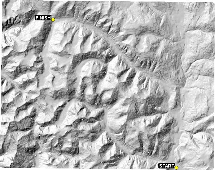
Figure 9.9 – The shaded relief terrain image we will route through
Just looking at the terrain, there are two paths that follow low-elevation routes without much change in direction. These two routes are illustrated in the following screenshot:
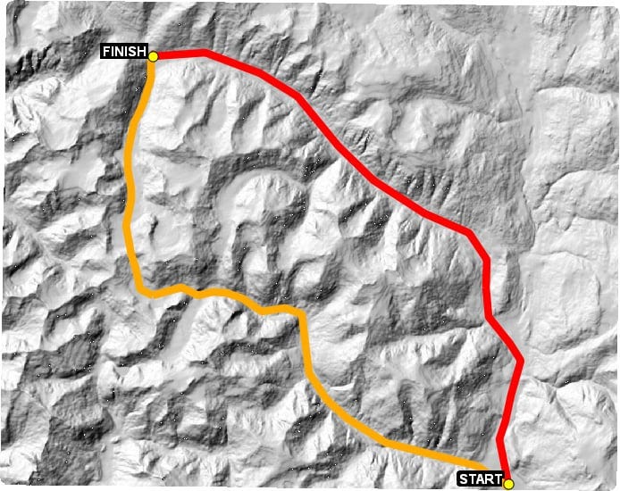
Figure 9.10 – Two obvious possible paths through the terrain
So, we would expect that when we use the A* algorithm, the result would be close. Remember that the algorithm only looks in the immediate vicinity, so it can’t look at the whole image as we can, and it can’t make adjustments early in the route based on a known obstacle ahead.
We will expand this implementation from our simple example and use Euclidean distance, or as the crow flies measurements, and we will also allow the search to look in eight directions instead of four. We will prioritize terrain as the primary decision point. We will also use distances, both to the finish and from the start, as lower priorities in order to make sure that we are moving forward toward the goal and not getting too far off track. Other than those differences, the steps are identical to the simple example. The output will be a raster with the path values set to one and the other values set to zero.
Now that we understand the problem, let’s solve it!
Loading the grid
We’ll start loading our ASCII grid terrain data using NumPy with the following steps:
First, we import necessary libraries such as NumPy for array operations, math for mathematical functions, linecache for reading specific lines from a file, and pickle for serializing Python objects:
import numpy as np
import math
from linecache import getline
import pickle
Next, we define the source file for the terrain data and the target file for the raster path. We then load the terrain data into a NumPy array, skipping the first six rows as they contain header information:
source = "dem.asc"
target = "path.asc"
cost = np.loadtxt(source, skiprows=6)
Then, we parse the header to obtain metadata such as the number of columns, rows, cell size, and nodata value:
hdr = [getline(source, i) for i in range(1, 7)]
values = [float(ln.split(" ")[-1].strip()) for ln in hdr]
cols, rows, lx, ly, cell, nd = values
Finally, we set the starting and ending positions on the grid:
sx = 1006
sy = 954
dx = 303
dy = 109
Now that we have our data, let’s set up the functions we’ll need to process it.
Defining the helper functions
We’ll need a couple of helper functions, as shown next, to calculate the score of each move:
We define a function called e_dist to calculate the Euclidean distance between two points:
def e_dist(p1, p2):
x1, y1 = p1
x2, y2 = p2
distance = math.sqrt((x1-x2)**2+(y1-y2)**2)
return int(distance)
Next, we define another function called weighted_score to calculate the weighted score for each node based on its distance from the start and end points as well as its elevation:
def weighted_score(cur, node, h, start, end):
cur_h = h[cur]
cur_g = e_dist(cur, end)
cur_d = e_dist(cur, start)
node_h = h[node]
node_g = e_dist(node, end)
node_d = e_dist(node, start)
score = 0
if node_h < cur_h:
score += cur_h-node_h
if node_g < cur_g:
score += 10
if node_d > cur_d:
score += 8
return score
We can now implement the A* algorithm.
The real-world A* algorithm
This algorithm is more complex than the simple version in our previous example. We use sets to avoid redundancy. It also implements our more advanced scoring algorithm and checks to make sure we aren’t at the end of the path before doing additional calculations. Unlike our last example, this more advanced version also checks cells in eight directions, so the path can move diagonally:
We define the astar function to implement the A* algorithm:
def astar(start, end, h):
Inside this function, we initialize sets for the closed set of nodes, the open set of nodes, and the path:
closed_set = set()
open_set = set()
path = []
Then, we add the starting point to the open set and enter a while loop that continues until the open set is empty:
open_set.add(start)
while open_set:
Within the loop, we pop a node from the open set and check whether it’s the endpoint. If it is, we return the path:
cur = open_set.pop()
if cur == end:
return path
Next, we add the current node to the closed set and the path:
closed_set.add(cur)
path.append(cur)
Then, we identify the neighbors of the current node and check whether the endpoint is among them. If it is, we return the path:
options = []
y1 = cur[0]
x1 = cur[1]
if y1 > 0:
options.append((y1-1, x1))
if y1 < h.shape[0]-1:
options.append((y1+1, x1))
if x1 > 0:
options.append((y1, x1-1))
if x1 < h.shape[1]-1:
options.append((y1, x1+1))
if x1 > 0 and y1 > 0:
options.append((y1-1, x1-1))
if y1 < h.shape[0]-1 and x1 < h.shape[1]-1:
options.append((y1+1, x1+1))
if y1 < h.shape[0]-1 and x1 > 0:
options.append((y1+1, x1-1))
if y1 > 0 and x1 < h.shape[1]-1:
options.append((y1-1, x1+1))
if end in options:
return path
We score the neighbors and add the best-scoring neighbor to the open set:
best = options[0]
best_score = weighted_score(cur, best, h, \
start, end)
for i in range(1, len(options)):
option = options[i]
if option in closed_set:
continue
option_score = weighted_score(cur,\
option, h, start, end)
if option_score > best_score:
best = option
best_score = option_score
open_set.add(best)
Now we can use the A* algorithm to create a path.
You can unlock the rest of this chapter that covers the entire real-world example of performing least cost path analysis, along with creating a normalized difference vegetation index (NDVI), a flood inundation model, and a color hillshade; converting the route to a shapefile; routing along streets; geolocating photos; and calculating satellite image cloud cover, for just $3. Packt subscribers can continue reading for free.
And that’s a wrap.
We have an entire range of newsletters with focused content for tech pros. Subscribe to the ones you find the most useful here. The complete PythonPro archives can be found here.
If you have any comments or feedback, take the survey or leave your thoughts below!
See you next week!